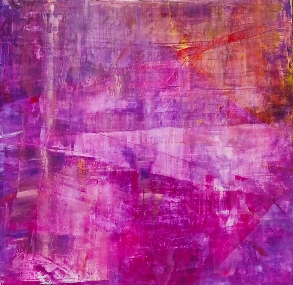
“Simulated Topological Edge States & Phase Boundary” Acrylic on plywood 1.2×1.2 x0.05m Horus9X! copyright 2026 northern hemisphere
With its intense gradients of magenta, violet, and intersecting horizontal and vertical bands, a mathematical heatmaps used to track quantum state transitions and particle interactions in a high-energy lattice simulator
System Architecture Diagram Mapping
Here is how the distinct visual fields and overlapping textures of artwork map directly to a high-energy quantum simulation lattice:
 TOPOLOGICAL BULK                CHIRAL SYMMETRY LAYER           TOPOLOGICAL EDGE STATES
+-----------------------+          +--------------------+          +-----------------------+

|                       |          |                    |          |                       |
|  Zone 1: Upper Deep   | =======> |  Zone 2: Mid-Band  | =======> |  Zone 3: Lower Intense |
|  Purple Grid          |  (Flux)  |  Phase Boundary    |  (Decay) |  Magenta Clusters     |
|  (Quantum Vacuum Matrix)         |  (Chiral Interface)|          |  (Protected Edge Mode)|
|                       |          |                    |          |                       |
+-----------------------+          +--------------------+          +-----------------------+
            ||                                                                 ||
            +==================================================================+
Quantum Coherence Feedback Loop- The Upper Deep Purple Grid (The Quantum Vacuum Matrix): The top half of painting features a dark, heavily textured grid where horizontal and vertical lines collide. This maps to the gauge field lattice. The grid squares represent discrete points in spacetime where virtual quarks and gluons interact, establishing the “bulk” of the quantum system.
- The Lighter Mid-Band (The Chiral Interface Phase Boundary): The bright, horizontally sheared band slicing through the center of the canvas illustrates a topological phase boundary. This is the critical threshold where the quantum system switches states. The shifting opacity simulates the loss of local symmetry as particles transition from one phase to another.
- The Intense Magenta Clusters (Protected Topological Edge States): The lower third of the painting erupts into highly saturated, intense magenta and pink tones. In quantum simulations, these concentrated visual bursts depict localized energy concentrations. Because they are “topologically protected,” they remain bright and stable against noise, resisting the decay seen in the upper layers.
- The Layered Textures and Scrapes (Quantum Fluctuations): The visible strokes and underlying scrapes across the entire canvas map perfectly to sub-atomic fluctuations. Instead of a static image, the varied thickness of the paint layers visualizes probability densities over simulated timeline steps.
For future use
The code models a 2D topological lattice (like a Su-Schrieffer-Heeger or Chern insulator variant) where localized edge states form at the boundary, generating the intense energy concentrations seen at the bottom of canvas.
import numpy as np
import matplotlib.pyplot as plt

# 1. Define Lattice Grid Size
Nx, Ny = 100, 100
X, Y = np.meshgrid(np.linspace(-3, 3, Nx), np.linspace(-3, 3, Ny))

# 2. Simulate the Background Quantum Vacuum Matrix (Upper Grid)
# Creates the underlying quantum fluctuations and grid-like noise
vacuum_fluctuations = np.sin(5 * X) * np.cos(5 * Y) * 0.15
quantum_noise = np.random.normal(0, 0.05, (Ny, Nx))
zone_1_bulk = vacuum_fluctuations + quantum_noise

# 3. Simulate the Phase Boundary (Lighter Mid-Band Shift)
# A transition zone modeling the broken chiral symmetry across the center
phase_boundary = np.exp(-((Y - 0.2) ** 2) / 0.1) * 0.4

# 4. Simulate Topologically Protected Edge States (Lower Intense Clusters)
# Localized, high-intensity energy states that resist decay at the boundary
# Shifted downward (Y = -1.5) to match the heavy magenta base of your canvas
edge_state_1 = np.exp(-((X - 1.0)**2 + (Y + 1.5)**2) / 0.8) * 1.5
edge_state_2 = np.exp(-((X + 1.2)**2 + (Y + 1.8)**2) / 0.5) * 1.2
zone_3_edge = edge_state_1 + edge_state_2

# 5. Composite the Total Wavefunction Probability Density
# Combining the fields to mimic the structural layers of the artwork
total_field = zone_1_bulk + phase_boundary + zone_3_edge

# 6. Plotting with a Customized Color Palette Matching Your Painting
plt.figure(figsize=(8, 8))
plt.imshow(
    total_field,
    extent=[-3, 3, -3, 3],
    origin='lower',
    cmap='plasma',      # 'plasma' perfectly captures the deep violets to hot magentas
    interpolation='bilinear'
)

# Visualizing the structure
plt.title("Simulated Topological Edge States & Phase Boundary", fontsize=12, pad=15)
plt.xlabel("Lattice X-Axis (Spatial Dimension)")
plt.ylabel("Lattice Y-Axis (Boundary Depth)")
plt.colorbar(label="Probability Density $|\\psi|^2$")
plt.grid(color='white', linestyle='--', linewidth=0.3, alpha=0.5)

plt.tight_layout()
plt.show()
Technical Mapping of the Code Objects:
zone_1_bulk: Controls the background grid frequencies. Increasing the multiplier innp.sin(5 * X)will make the upper “scrapes” tighter and more dense.phase_boundary: Controls the center horizontal tear. Changing theY - 0.2value moves the light streak higher or lower across the canvas.zone_3_edge: Dictates the placement of the hot pink/white glare points. Adding more exponential equations here lets you place additional bright nodes anywhere on the lattice.
stable assistant take